How To Fix Number Error In Excel

What are Errors In Excel?

MS Excel is a powerful tool that enables users to tape massive data sets in cells defined past row and column coordinates. It'due south easy-to-employ features and avant-garde functions assist users in manipulating their recorded information and achieving the required output in their desired format. Nonetheless, when applying a formula to the worksheet, we may get an unexpected error code. Such errors in Excel indicate the probable mistakes in our functions and what we can do to resolve them.

But first, to ensure we can view all the errors in our worksheet,

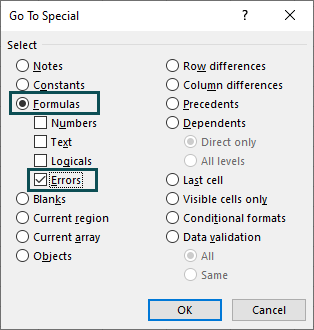
• Navigate through Habitation > Find & Select > Become To Special or employ the shortcut keys Ctrl + Chiliad and click on Special.
• The Become To Special window appears. Then, under Formulas, check the box against Errors and click OK.

At present that we can find errors in Excel, permit u.s. learn how toset errors in excel.

For instance, nosotros accept a table showing the yearly incomes in column A. Now, nosotros need to determine the monthly earnings in column B by dividing each annual income past 12. Nonetheless, while applying the formula in cell B3, we carve up the numerator by 0 instead of 12. As a result, nosotros will get an error as depicted below:

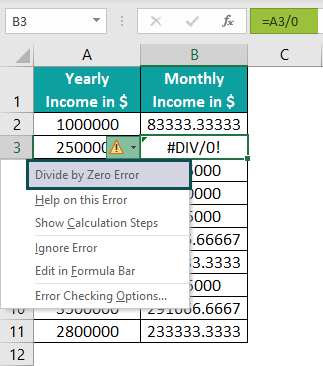
The jail cell with the fault code will take a small green triangle in the top-left corner.

Nosotros will get a yellowish diamond icon with an assertion mark when nosotros click on this cell.

Also, if we hover our mouse cursor over the icon, a hover text volition appear explaining the reason for the error.

In addition, when we click on the icon, we will get a menu with options to handle the error according to our requirements.

And then, nosotros tin find errors in excel. At present, allow us learn how to set errors in excel.

Table of contents

• What are Errors In Excel?
  • List Of Top 10 Errors In Excel
    • 1) #DIV/0
    • 2) #N/A
    • 3) #Proper name?
    • 4) #NULL!
    • 5) #NUM!
    • 6) #REF!
    • 7) #VALUE!
    • viii) #####
    • nine) Circular Reference
    • 10) #SPILL!
  • Conclusion
  • Download Template
  • Recommended Articles

List Of Top 10 Errors In Excel

Hither are the superlative 10 types of errors in Excel which we will typically encounter while working on MS Excel.

Consider the tabular array below:

Let united states understand each error code we might get while applying different formulas to the to a higher place table data.

one) #DIV/0

Description

Nosotros volition see the error code #DIV/0 when the formula we employ in a prison cell tries to divide an empty cell or if the value of the jail cell is 0.

On the other manus, if nosotros attempt to detect the boilerplate of empty cells or not-numerical values, so over again, we will get the #DIV/0 error.

How To Fix?

Firstly,

• Ensure the cells used and referred to in the formula is right and contains valid data.
• Check whether the cell references in excel we utilise to carve up other data values are not blank or contains 0.
• See the cells referred to in the formula does not display the #DIV/0 fault code.

Yet, the best way to fix the #DIV/0 mistake is by using the IF() function and IFERROR() part. These evaluate the denominator for 0 or bare cells.

And, when nosotros use these functions, nosotros tin ensure that we do not see the mistake lawmaking. Instead, the output will be 0 or a statement that we tin brandish in the cell every bit the outcome of the function, letting the user know what to exercise to go the correct respond.

Case

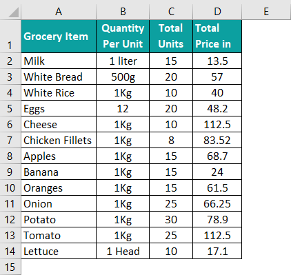
Consider the beneath table listing the grocery items and units sold. Now, let us add a column that shows the Charge per unit Per Unit of measurement in $, obtained by dividing the total price by the total units. Clearly, we can run into that the full units of tomatoes are missing from the table.

Pace 1: Choose cell E2 and enter the formula for dividing the total prices past the total units.

Step 2: In one case we drag the fill up handle downwards and copy the formula in cells C3:C14, the expression in prison cell E13 will become =D13/C13.

So, the output will be:

The #DIV/0 mistake occurs for the detail, Tomato as the formula divides the full price (0) by 0. And so, hither is how nosotros can employ the IFERROR() in cavalcade Due east and avert #DIV/0 fault. The formula in cell E13 is =IFERROR(D13/C13,"").

The formula at present shows the rate per unit for every item. And in this case, information technology checks the denominator for 0 or spaces to return a bare cell, every bit in cell E13.

Alternatively, the IF() formula in cell E13 (used to avoid the #DIV/0 error) will be

=IF(C13=0,"",D13/C13)

The function checks for 0 or blank cells in column C, every bit the cells in column C are the denominators in the formula. And then, the cells in column E will be blank if the corresponding cell values in column C are 0 or empty.

ii) #Northward/A

Clarification

The #N/A error code implies that a value is not available. It typically occurs when we use lookup functions, such as VLOOKUP, HLOOKUP, and Lucifer excel function.

Ideally, when nosotros effort looking up a value in a column to display its data, we will get the #N/A mistake when the lookup value is not present in the specific column. The error likewise occurs due to actress spaces or misspelled data in the formula.

How To Gear up?

As the beginning pace, perform a sanity check of our lookup table.

• Check for extra spaces and incorrect spellings in the lookup value and the table.
• Ensure the lookup table is complete
• Next, the lookup value and the table should have the same data types.
• Also, the exact friction match configuration should be correct.

The IFERROR() and IFNA() can help the states ready errors in excel. Nosotros can nest our LOOKUP and Lucifer excel functions in them and ensure nosotros do not get the fault code in our results. Then, instead of seeing the #N/A error, our output will show space or a meaningful comment, thus improving information technology.

Example

Suppose we want to display the full cost for certain items on another table, say Corn and Cheese. We get the below output as shown in the image beneath:

We await up the total prices for Cheese and Corn in the second tabular array, from the beginning one, using the formulas shown in cells I3 and I4.

However, the function returns the error #N/A for both items. On checking closely, we find an extra infinite before the lookup value, Cheese, in the second table. And Corn is not available on the first tabular array'southward grocery list.

Stride 1: Remove the additional space before the lookup value, Cheese, in jail cell G3. The output will be:

Pace 2: Use IFERROR() with the VLOOKUP() to remove the #N/A fault and provide a more than meaningful output for the item not bachelor. The formula in cell I4 will be:

=IFERROR(VLOOKUP(G4,A:D,4,0),"Item Not Available")

The higher up formula volition return the output Item Not Bachelor even if nosotros incorrectly type the part name VLOOKUP. On the other hand, the IFNA() is a function that exclusively fixes the #N/A error. The formula in cell I4 volition exist:

=IFNA(VLOOKUP(G4,A:D,four,0),"Particular Non Bachelor")

iii) #Name?

Clarification

If Excel does not recognize any part of the formula such as the function name, syntax, cell references, or value in a cell, we volition see the error #Name?.

Typically, we volition get this error when nosotros misspell the office proper noun, miss a colon, refer to a name not defined, or provide a text value without double quotations. The mistake can also occur when we use a role requiring an add together-in, merely we practise not enable the add together-in.

How To Fix?

Using the Formula Sorcerer is a straightforward way to overcome role proper noun typo errors in Excel. Once we start entering the function name in a cell or the Formula Bar, Excel will list the functions starting with the entered word. And when nosotros click on the required function or enter the open parenthesis, the Formula Wizard volition bear witness the syntax as hover text.

Alternatively, we can select the jail cell with the formula and choose Formulas > Insert Part. It will open up the Function Arguments window, where we can cheque and correct the syntax errors.

Example

Let us assume that the data for the vegetables are non available in the Grocery Items table. So, permit us ascertain a proper name for the cell range A1:C14 equally Grocery_Item_Total_Units, using the below steps:

Pace 1: Select the jail cell range A1:C14 and choose Formulas > Define Name > Define Proper name.

Stride two: Enter the proper name as Grocery_Item_Total_Units in the New Name window. And and so, click OK.

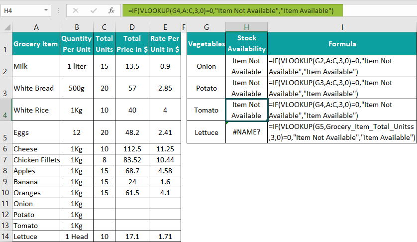
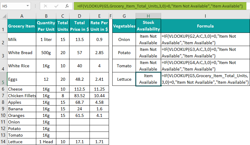
For example, if nosotros need to cheque the stock availability for the vegetables in the grocery item list, we will apply the IF() and VLOOKUP() to determine the output, equally depicted below:

The output in cavalcade H should be 'Detail Not Available' for the first three items in column G and 'Item Bachelor' for Lettuce. Yet, when applying the formulas (refer to the column I), we will see the error #NAME? for all iv vegetables. Permit us understand how toprepare errors in excel.

Step 1: The formula in cell H2 has a typo fault. Right the IF() name from IIF to IF to get the below output.

Step 2: The VLOOKUP() is missing a colon in the cell range. Insert a colon betwixt A and C column references to go the correct output.

Step 3: The text outputs in the IF(), Particular Not Available and Item Bachelor, are not in double quotations. Thus, put them in double quotes to remove the error #NAME?.

Step 4: The VLOOKUP() in prison cell H5 uses the defined name for the A:C cell range. Only the spelling is incorrect. In one case we update the defined proper name correctly, the mistake #Proper noun? will get fixed.

4) #NULL!

Description

The #Cypher! error appears when we utilise a infinite in place of the specific intersection operator, such equally a colon or comma, in cell ranges and references. The fault likewise occurs if we enter a space instead of the required mathematical operator between cell references.

How To Fix?

Here are a few checks we can perform to prepare errors in excel.

• Ensure we enter the required mathematical operators betwixt the specific cell references.
• A cell range should take a colon in betwixt to denote the intersection between the get-go and finish points in the cell range.
• Ensure the formula has comma-separated private cell references.

Instance

Suppose nosotros want to determine the overall total units of all items and those of fruits from the Grocery Items table. We tin create ii tables and using the SUM() (shown in cells H2 and K2), we can calculate the required values in each table, as depicted beneath:

However, we get the #NULL! error in both the tables. The steps used to fix errors in excel are equally follows:

Pace one: The cell range in the prison cell G2 SUM() has a space in between and is missing a colon. Remove the space, insert a colon, and press Enter to achieve the required output.

Step ii: The SUM() in jail cell J2 is missing a comma in between the cell references C9 and C10. Instead of the comma, at that place is a space. Thus, remove the space, insert a comma between prison cell references C9 and C10 and press the Enter key to fix the fault.

5) #NUM!

Description

We get the #NUM! error when we enter a numeric value equally an argument in a office or in a format that it does not support.

The following reasons show when nosotros get #NUM! error.

• The function output is also large.
• Statement in the function is incorrect.
• The mathematical calculation is not possible to perform.
• The iteration functions, such as RATE(), cannot observe the output after multiple iterations.

How To Fix?

We tin fix the #NUM! error by:

• Identifying the error cells and adjusting the argument values as required in the formula.
• Ensuring the entered arguments have the proper formats, as required in the formula.

We tin besides use the IFERROR() to remove the #NUM! error and evidence a meaningful output.

Instance

Assume the rate per unit of White Rice will grow exponentially by 600.

Pace 1: Enter the beneath formula in cell H2.

=E4^600

Just since the output is too large, we will run across the below error.

Step 2: Instead, nosotros can use the IFERROR() to display a more meaningful comment, as depicted below:

=IFERROR(E4^600,"Too large a number")

All the same, a more common scenario for getting the #NUM! error is when we attempt to observe the square root of a negative number. In such a case, we need to use the ABS() nested in the SQRT().

The syntax volition be:

=SQRT(ABS(value))

As well, to ensure that the iteration functions practice not return the #NUM! error, first choose File > Options > Formulas. Then, under Calculation options, check the box against Enable iterative calculation and adjust the Maximum Iterations and Maximum Change values.

While the beginning one should take a higher value, the second parameter needs to exist small. Such settings will ensure more iterations and more than accurate output without the #NUM! error.

half-dozen) #REF!

Description

We will get the #REF! error if a jail cell reference we use in our formula is invalid. Such errors in Excel occur when the referenced prison cell gets deleted. Another scenario is we copy a formula with relative cell references in another location where the references are not valid.

The mistake also occurs when nosotros enter an wrong table_array in a VLOOKUP() or alphabetize lookup range in the INDEX().

How To Fix?

Here are a few solutions we can check.

• Using Excel'southward undo option, recover the deleted row or column cells.
• Re-enter the deleted data and update the cell references in the formula.

Too, equally in the case of other errors in Excel, we tin can remove #REF! mistake using the IFERROR(), especially when developing cell references dynamically with the INDIRECT().

Example

Suppose the Grocery Items table has another cavalcade, Item ID, appended earlier the Grocery Item column. Nosotros use the INDEX excel function to decide the total price of the item with ID R085.

Step 1: Enter the Alphabetize() in cell J2.

=INDEX(A1:E14,9,5)

At present, assume we accidentally deleted the Item ID cavalcade. The output will become:

The index lookup range changes automatically from A1:E14 to A1:D14, and nosotros get the #REF! error in cell I2. We can immediately apply the shortcut keys Ctrl + z. It will undo the delete activity and fix the fault.

Similarly, if we enter the row or column range incorrectly, say, we entered xv as the row range instead of 9 in the Index(), the output becomes:

Nosotros tin manually correct the cell references in the formula to get the correct output.

Otherwise, nosotros will meet a bare cell instead of the error when using the IFERROR() with the INDEX() containing the incorrect lookup range.

7) #VALUE!

Description

When nosotros enter an argument in a formula, which does not accept the required data blazon, the function volition return #VALUE! mistake. The error indicates nosotros take typed our expression incorrectly, or at that place is an outcome with the prison cell references nosotros used in our formula.

It typically happens when we enter a text when the office requires a numeric value every bit input or i that should take a Date type.

Here are a few facts that we can cheque:

How To Fix?

• Cheque our formula past selecting the prison cell with the function and choosing Formulas > Evaluate Formula > Evaluate. Then, we tin check the pace-by-footstep evaluation and determine the fault source.
• Check and remove the extra spaces in cells whose values might cause the error.
• Check for special characters and text in cells causing the fault.
• Instead of typing in the formulas with mathematical formulas, use the Excel built-in functions.
• Apply the IFERROR() to replace the error with a more meaningful part return value.

Example

Consider we have iii new columns in the Grocery Items table. The commencement two columns testify each item's stock gild and receive dates. And the third column determines the waiting period during the stock arrival.

Presume we used the DATEDIF() to decide the waiting period.

Step 1: Enter the DATEDIF() formula in cell H2 and elevate the fill handle downward to copy the formula in cells C3:C14. And then, the formula in prison cell H10 will be:

=DATEDIF(F10,G10,"D")

In the table higher up, prison cell H10 shows the #VALUE! error equally the Stock Receive Date for Oranges is NA, a text instead of a valid engagement.

Footstep ii: Either we right the entry in jail cell G10 to become the right event, or we can use the IFERROR() to supervene upon the mistake with an apt annotate. The outputs in the two scenarios volition be:

viii) #####

Clarification

If we run into a row of # (hash symbol) in a cell, information technology indicates a hashtag error. Notwithstanding, it is not an error; it suggests that the column width is non adequately wide to show the cell content.

We will get the hashtag error when:

• We enter a numeric value or text information exceeding a limit of 253 characters in a cell that stores numbers, dates, or fourth dimension.
• We enter a negative value in a jail cell that stores numbers, dates, or fourth dimension.
• We enter a formula whose return value exceeds the cell column width.

How To Fix?

When we see the ##### error:

• Increase the prison cell column width.
• Reduce the cell data length or change the prison cell format type to General.
• Right the prison cell value or the function that returns an incorrect value.

Example

For example, the Stock Gild Date format is 24-hour interval, Month Date, Yr in the Grocery Items tabular array.

Step 1: Choose column F and select Dwelling > Date > More Number Formats.

Step 2: In the Format Cells window, choose Appointment and the required date format as depicted beneath.

When we click OK, the table will announced as shown in the epitome below:

As the cavalcade F width is shorter, we will get the ##### mistake.

Step three: Increase the column F width to make the table error-complimentary.

9) Circular Reference

Description

A circular reference error appears when a function refers to its own cell. The jail cell reference can exist direct or indirect, building endless loops of evaluations.

In the case of the direct circular reference, we will utilise a reference to the prison cell containing the formula directly within the function. On the other manus, when a function refers to a prison cell containing a circular reference, it is a scenario of indirect circular reference.

How To Set?

We can trace the round reference in excel to the source to correct the initial formula or remove the reference stage by stage.

Excel offers two ways to trace the relationship between functions and cells to remove the circular reference, which are:

• Trace Precedents – It helps in tracking cells that affect the active prison cell.
• Trace Dependents – It helps track cells that depend on the electric current prison cell.

Nosotros can find the above options in the Formulas tab in the Excel ribbon.

Case

Let usa consider the data for Milk, White Bread, Eggs, and Cheese from the Grocery Items table. And suppose we demand to go the product of Total Units and Full Price for these four items to calculate the Overall Total Toll in cell G10.

Pace 1: Enter the SUM() in jail cell G7. Suppose we provide an incorrect cell range, G2:G7 instead of G2:G5. The formula in prison cell G7 will exist:

=SUM(G2:G7)

As we enter the SUM() in cell G7 and employ a reference to G7 in the formula, nosotros volition run across the below warning message about circular reference when we press the Enter cardinal.

When we click OK, the function returns 0 as the output.

Stride 2: Using the SUM() in cell H7, calculate the total cost for the iv items with the formula =SUM(H2:H5).

Step 3: Get the production of values in cells G7 and H7 in prison cell G10. It will be 0.

We need to correct the circular reference error to become the correct output.

Footstep 4: Choose Formulas > Error Checking > Circular Reference.

Information technology shows which source cell has a circular reference. So now, we tin correct the error by providing the right cell range in the SUM() in jail cell G7.

Pace 5: Change the cell range in the SUM() in prison cell G7 as G2:G5.

So, the formula is =SUM(G2:G5)

Once nosotros right the cell range used in the SUM() in cell G7, nosotros will go the right output in prison cell G10.

10) #SPILL!

Description

We will see the #SPILL! mistake when the formula nosotros entered in a cell returns multiple results, only Excel does not return the output to the respective filigree.

In other words, the function returns a spill range, evaluating through a jail cell that already contains data.

How To Fix?

• Commencement, identify the cells creating the hindrance and blocking the office from execution.
• Next, clear the values from the obstructing cells.

We will discover the formula output shows up in the required cells.

Example

Suppose we wish to create another cavalcade Grocery Items_New with the first seven items from the Grocery Items tabular array followed by a listing of new essentials.

Step 1: In cavalcade H with the heading Grocery Item_New, enter the new items from jail cell H8:H14.

Also, the UNIQUE() in cell G2 is:

=UNIQUE(A2:A8)

We volition become the #SPILL! error as the cell range nosotros chose, A2:A8, overlaps with the G8 value, Cherries. Information technology means that the spill range is not blank.

Step 2: Delete the cell G8 value, and immediately the array will spill, filling the cells from G2:G8, every bit depicted below:

Conclusion

To summarize, the Errors in Excel assist identify where we might take gone incorrect while performing calculations in our worksheets. Nosotros will notice them useful, especially when working with massive data sets.

So, empathize them thoroughly to brand the necessary corrections in your calculations and accomplish your desired results.

Download Template

This article must be helpful to understandErrors in Excel, with examples. Y'all can download the template here to employ it instantly.

Recommended Articles

This has been a guide to Errors in Excel. Here nosotros talk over the listing of summit 10 errors in excel & how to fix them with examples and downloadable excel template. Y'all tin learn more from the following articles –

• Mixed References In Excel
• Alternatives to VLOOKUP In Excel
• Track changes in Excel

Source: https://www.excelmojo.com/errors-in-excel/

Share this post